Dynamic Programming

Matrix Chain-Products

Dynamic Programming is a general algorithm design paradigm.
- Rather than give the general structure, let us first give a motivating example:
- Matrix Chain-Products
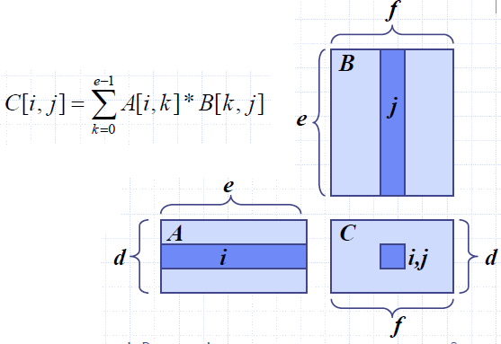
Review: Matrix Multiplication.
- C = A*B
- A is d × e and B is e × f
- O(d⋅e⋅f ) time

Dynamic_Programming_Matrix_Product

Matrix Chain-Product:
- Compute A=A0*A1*…*An-1
- A_i is d_i × d_i+1
- Problem: How to parenthesize?
Example
- B is 3 × 100
- C is 100 × 5
- D is 5 × 5
- (B*C)*D takes 1500 + 75 = 1575 ops
- B*(C*D) takes 1500 + 2500 = 4000 ops

Enumeration Approach

Matrix Chain-Product Alg.:
- Try all possible ways to parenthesize A=A0*A1*…*An-1
- Calculate number of ops for each one
- Pick the one that is best
Running time:
- The number of parenthesizations is equal to the number of binary trees with n nodes
- This is exponential!
- It is called the Catalan number, and it is almost 4n.
- This is a terrible algorithm!

Greedy Approach

Idea #1: repeatedly select the product that uses (up) the most operations.
Counter-example:
- A is 10 × 5
- B is 5 × 10
- C is 10 × 5
- D is 5 × 10
- Greedy idea #1 gives (A*B)*(C*D), which takes 500+1000+500 = 2000 ops
- A*((B*C)*D) takes 500+250+250 = 1000 ops

Another Greedy Approach

Idea #2: repeatedly select the product that uses the fewest operations.
Counter-example:
- A is 101 × 11
- B is 11 × 9
- C is 9 × 100
- D is 100 × 99
- Greedy idea #2 gives A*((B*C)*D)), which takes 109989+9900+108900=228789 ops
- (A*B)*(C*D) takes 9999+89991+89100=189090 ops
- The greedy approach is not giving us the optimal value.

“Recursive” Approach

Define subproblems:
- Find the best parenthesization of A_i*A_i+1*…*A_j.
- Let N_i,j denote the number of operations done by this subproblem.
- The optimal solution for the whole problem is N_0,n-1.
Subproblem optimality: The optimal solution can be defined in terms of optimal subproblems
- There has to be a final multiplication (root of the expression tree) for the optimal solution.
- Say, the final multiply is at index i: (A₀*…*A_i)*(A_i+1*…*A_n-1).
- Then the optimal solution N_0,n-1 is the sum of two optimal subproblems, N_0,i and N_i+1,n-1 plus the time for the last multiply.
- If the global optimum did not have these optimal subproblems, we could define an even better “optimal” solution.

Characterizing Equation

The global optimal has to be defined in terms of optimal subproblems, depending on where the final multiply is at.
Let us consider all possible places for that final multiply:
- Recall that A_i is a d_i × d_i+1 dimensional matrix.
- So, a characterizing equation for N_i,j is the following:

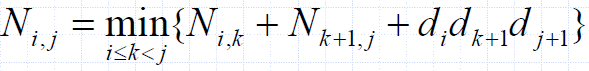
Dynamic_Programming_Matrix_Characterizing_Equation

Note that subproblems are not independent–the subproblems overlap.

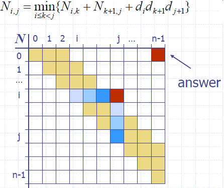
Dynamic Programming Algorithm Visualization

The bottom-up construction fills in the N array by diagonals
N_i,j gets values from previous entries in i-th row and j-th column
Filling in each entry in the N table takes O(n) time.
Total run time: O(n³)
Getting actual parenthesization can be done by remembering “k” for each N entry

Dynamic_Programming_Matrix_DP

Dynamic Programming Algorithm

Since subproblems overlap, we don’t use recursion.
Instead, we construct optimal subproblems “bottom-up.”
N_i,i’s are easy, so start with them Then do problems of “length” 2,3,… subproblems, and so on.
Running time: O(n³)

Algorithm matrixChain(S):
Input: sequence S of n matrices to be multiplied
Output: number of operations in an optimal parenthesization of S
for i ← 1 to n − 1 do
  Ni,i ← 0
for b ← 1 to n − 1 do
  { b = j − i is the length of the problem }
  for i ← 0 to n − b − 1 do
    j ← i + b
    Ni,j ← +∞
    for k ← i to j − 1 do
      Ni,j ← min{Ni,j, Ni,k + Nk+1,j + di dk+1 dj+1}
return N0,n−1

The General Dynamic Programming Technique

Applies to a problem that at first seems to require a lot of time (possibly exponential), provided we have:
- Simple subproblems: the subproblems can be defined in terms of a few variables, such as j, k, l, m, and so on.
- Subproblem optimality: the global optimum value can be defined in terms of optimal subproblems
- Subproblem overlap: the subproblems are not independent, but instead they overlap (hence, should be constructed bottom-up).

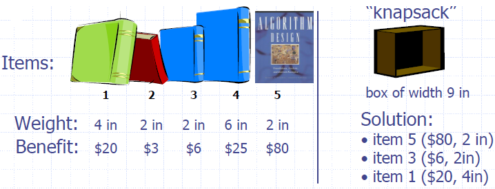
The 0/1 Knapsack Problem

Given: A set S of n items, with each item i having
- w_i - a positive weight
- b_i - a positive benefit
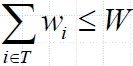
Goal: Choose items with maximum total benefit but with weight at most W.
If we are not allowed to take fractional amounts, then this is the 0/1 knapsack problem.
In this case, we let T denote the set of items we take
Objective: maximize
Constraint:

Example

Given: A set S of n items, with each item i having
- w_i - a positive “benefit”
- b_i - a positive “weight”
Goal: Choose items with maximum total benefit but with weight at most W.

A 0/1 Knapsack Algorithm, First Attempt

S_k: Set of items numbered 1 to k.
Define B[k] = best selection from S_k.
Problem: does not have subproblem optimality:
- Consider set S={(3,2),(5,4),(8,5),(4,3),(10,9)} of (benefit, weight) pairs and total weight W = 20

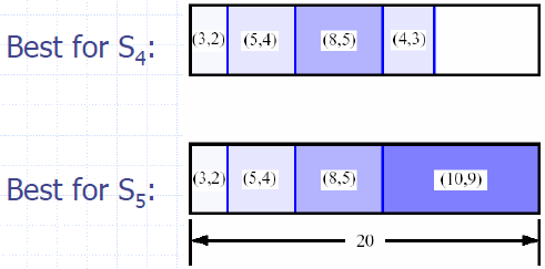
Dynamic_Programming_Knapsack_Example

A 0/1 Knapsack Algorithm, Second Attempt

S_k: Set of items numbered 1 to k.
Define B[k,w] to be the best selection from S_k with weight at most w
Good news: this does have subproblem optimality.
I.e., the best subset of S_k with weight at most w is either
- the best subset of S_k-1 with weight at most w or
- the best subset of S_k-1 with weight at most w−w_k plus item k

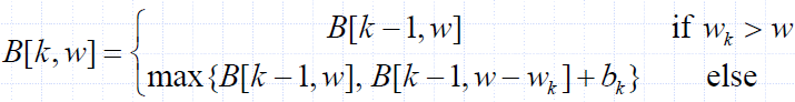
0/1 Knapsack Algorithm

Recall the definition of [k,w]
Since B[k,w] is defined in terms of B[k−1,*], we can use two arrays of instead of a matrix
Running time: O(nW).
Not a polynomial-time algorithm since W may be large
This is a pseudo-polynomial time algorithm

Algorithm 01Knapsack(S, W):
Input: set S of n items with benefit bi and weight wi; maximum weight W
Output: benefit of best subset of S with weight at most W
{let A and B be arrays of length W + 1}
for w ← 0 to W do
  B[w] ← 0
for k ← 1 to n do
  copy array B into array A
for w ← wk to W do
  if A[w−wk] + bk > A[w] then
    B[w] ← A[w−wk] + bk
return B[W]