Shortest Paths

Weighted Graphs

In a weighted graph, each edge has an associated numerical value, called the weight of the edge
Edge weights may represent, distances, costs, etc.
Example:
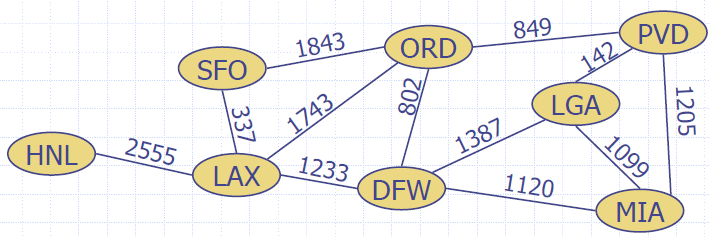
- In a flight route graph, the weight of an edge represents the distance in miles between the endpoint airports

Shortest_Path_Weighted_Graphs

Shortest Path Problem

Given a weighted graph and two vertices u and v, we want to find a path of minimum total weight between u and v.
- Length of a path is the sum of the weights of its edges.
Example:
- Shortest path between Providence and Honolulu
Applications: Internet packet routing, Flight reservations, Driving directions

Shortest Path Properties

Property 1:
- A subpath of a shortest path is itself a shortest path
Property 2:
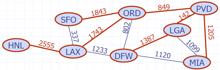
- There is a tree of shortest paths from a start vertex to all the other vertices
Example:
- Tree of shortest paths from Providence

Shortest_Path_Weighted_Graphs_Properties

Dijkstra's Algorithm

The distance of a vertex v from a vertex s is the length of a shortest path between s and v
Dijkstra’s algorithm computes the distances of all the vertices from a given start vertex s
Assumptions:
- the graph is connected
- the edges are undirected
- the edge weights are nonnegative
We grow a “cloud” of vertices, beginning with s and eventually covering all the vertices
We store with each vertex v a label d(v) representing the distance of v from s in the subgraph consisting of the cloud and its adjacent vertices
At each step
- We add to the cloud the vertex u outside the cloud with the smallest distance label, d(u)
- We update the labels of the vertices adjacent to u

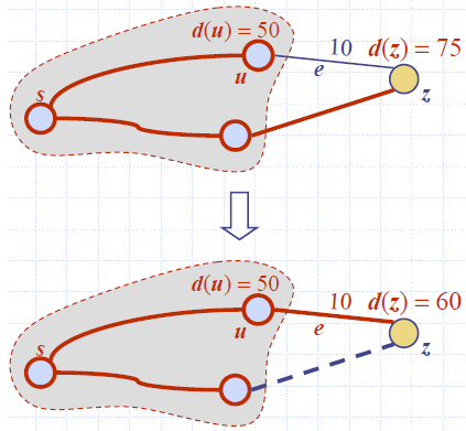
Edge Relaxation

Consider an edge e = (u,z) such that
- u is the vertex most recently added to the cloud
- z is not in the cloud
The relaxation of edge e updates distance d(z) as follows:
- d(z) ← min{d(z),d(u) + weight(e)}

Shortest_Path_Dijkstra

Example

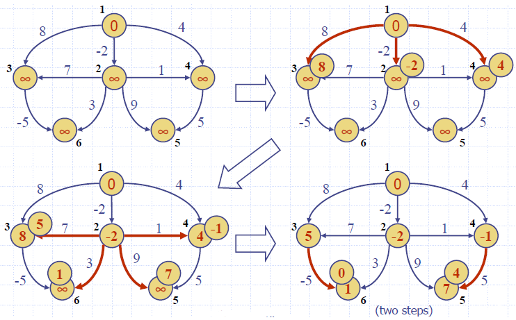
Shortest_Path_Dijkstra_Example

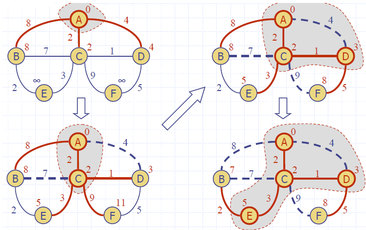
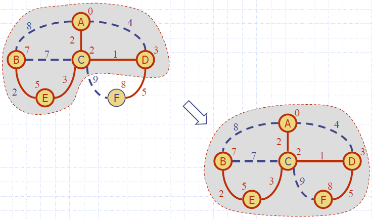
Dijkstra’s Algorithm

A priority queue stores the vertices outside the cloud
- Key: distance
- Element: vertex
Locator-based methods
- insert(k,e) returns a locator
- replaceKey(l,k) changes the key of an item
We store two labels with each vertex:
- Distance (d(v) label)
- locator in priority queue

Algorithm DijkstraDistances(G, s)
  Q ← new heap-based priority queue
  for all v ∈ G.vertices()
    if v = s
      setDistance(v, 0)
    else
      setDistance(v, ∞)
      l ← Q.insert(getDistance(v), v)
      setLocator(v,l)
    while ¬Q.isEmpty()
      u ← Q.removeMin()
      for all e ∈ G.incidentEdges(u)
        { relax edge e }
        z ← G.opposite(u,e)
        r ← getDistance(u) + weight(e)
        if r < getDistance(z)
          setDistance(z,r)
          Q.replaceKey(getLocator(z),r)

Analysis

Graph operations
- Method incidentEdges is called once for each vertex
Label operations
- We set/get the distance and locator labels of vertex z O(deg(z)) times
- Setting/getting a label takes O(1) time
Priority queue operations
- Each vertex is inserted once into and removed once from the priority queue, where each insertion or removal takes O(log n) time
- The key of a vertex in the priority queue is modified at most deg(w) times, where each key change takes O(log n) time
Dijkstra’s algorithm runs in O((n + m) log n) time provided the graph is represented by the adjacency list structure
- Recall that Σ_v deg(v) = 2m
The running time can also be expressed as O(m log n) since the graph is connected

Code

package examples;
import graphLib.*;
import graphTool.Algorithm;
import graphTool.Attribute;
import graphTool.GraphTool;

import java.awt.Color;
import java.io.Serializable;
import java.util.ArrayList;
import java.util.Arrays;
import java.util.Iterator;
import java.util.LinkedList;
import java.util.Random;


public class GraphExamples<V,E> {

       @Algorithm(vertex=true)
        public void dijkstra(Graph<V,E> g,Vertex<V> s, GraphTool<V,E> t){
    //-----------------------------------------------------------------


            t.show(g);
    //-----------------------------------------------------------------

            // sets the attribute 's' of each vertex 'u' from wich
            // we can reach 's' to the value 'g' where 'g' is the gateway
            // for 'u' on the shortest path from 'u' to 's'
            MyPriorityQueue<Double, Vertex<V>> pq = new MyPriorityQueue<>();
            Iterator<Vertex<V>> it = g.vertices();
            // put all vertices to pq and give them
            // an attribute Attribut.DISTANCE and PQLOCATOR
            while(it.hasNext()){
                Vertex<V> v = it.next();
                v.set(Attribute.DISTANCE,Double.POSITIVE_INFINITY);
                v.set(Attribute.string,"inf");
                Locator<Double,Vertex<V>> loc = pq.insert(Double.POSITIVE_INFINITY,v);
                v.set(Attribute.PQLOCATOR,loc);
                // v.set(Attribut.color, Color.red);
                t.show(g);
            }
            // correct the attributes for s
            s.set(Attribute.string,"0");
            s.set(Attribute.DISTANCE,0.0);
            t.show(g);
            pq.replaceKey((Locator<Double,Vertex<V>>)s.get(Attribute.PQLOCATOR),0.0);
            while( ! pq.isEmpty()){
                Vertex<V> u = pq.removeMin().element();    
                u.set(Attribute.color,Color.GREEN);
                if (u.has(Attribute.DISCOVERY)){
                    Edge<E> e = (Edge<E>)u.get(Attribute.DISCOVERY);
                    e.set(Attribute.color,Color.GREEN);
                    t.show(g);
                }

                // now make the relaxation step for all
                // neighbours:
                Iterator<Edge<E>> eIt;
                if (g.isDirected()) eIt = g.incidentInEdges(u); // backwards!
                else eIt = g.incidentEdges(u);
                while (eIt.hasNext()){
                    Edge<E> e = eIt.next();
                    double weight = 1.0; // default weight
                    //Original version: if (e.has(Attribut.weight)) weight = (Double)e.get(Attribut.weight);

                    //Whether the graph comes from graphexamples or not it has to be casted differently
                    if (e.has(Attribute.weight)) {
                       weight = (Double)e.get(Attribute.weight);
                    }
                    Vertex<V> z = g.opposite(e, u);
                    //Relaxation
                    double newDist = (Double) u.get(Attribute.DISTANCE);// +weight;
                    if (newDist < (Double)z.get(Attribute.DISTANCE)){
                        z.set(Attribute.DISTANCE,(Double)newDist);
                        z.set(Attribute.string,""+newDist);
                        z.set(Attribute.DISCOVERY,e);
                        z.set(s,u);
                        pq.replaceKey((Locator<Double,Vertex<V>>)z.get(Attribute.PQLOCATOR),newDist);
                        t.show(g);
                    }
                }
            }
            t.show(g);
        }

    /**
     * @param args
     *
     */
    public static void main(String[] args) {

        //         make an undirected graph
        IncidenceListGraph<String,String> g =
                new IncidenceListGraph<>(true);
        GraphExamples<String,String> ge = new GraphExamples<>();
        Vertex vA = g.insertVertex("A");
        vA.set(Attribute.name,"A");
        Vertex vB = g.insertVertex("B");
        vB.set(Attribute.name,"B");
        Vertex vC = g.insertVertex("C");
        vC.set(Attribute.name,"C");
        Vertex vD = g.insertVertex("D");
        vD.set(Attribute.name,"D");
        Vertex vE = g.insertVertex("E");
        vE.set(Attribute.name,"E");
        Vertex vF = g.insertVertex("F");
        vF.set(Attribute.name,"F");
        Vertex vG = g.insertVertex("G");
        vG.set(Attribute.name,"G");

        Edge e_a = g.insertEdge(vA,vB,"AB");
        Edge e_b = g.insertEdge(vD,vC,"DC");
        Edge e_c = g.insertEdge(vD,vB,"DB");
        Edge e_d = g.insertEdge(vC,vB,"CB");
        Edge e_e = g.insertEdge(vC,vE,"CE");
        e_e.set(Attribute.weight,2.0);
        Edge e_f = g.insertEdge(vB,vE,"BE");
        e_f.set(Attribute.weight, 7.0);
        Edge e_g = g.insertEdge(vD,vE,"DE");
        Edge e_h = g.insertEdge(vE,vG,"EG");
        e_h.set(Attribute.weight,3.0);
        Edge e_i = g.insertEdge(vG,vF,"GF");
        Edge e_j = g.insertEdge(vF,vE,"FE");
        GraphTool t = new GraphTool(g,ge);

        //    A__B     F
        //      /|\   /|
        //     / | \ / |
        //    C__D__E__G   
        //    \     /
        //     \___/
        //   
    }
}

Extension of Dijkstra

Using the template method pattern, we can extend Dijkstra’s algorithm to return a tree of shortest paths from the start vertex to all other vertices
We store with each vertex a third label:
- parent edge in the shortest path tree
In the edge relaxation step, we update the parent label

Algorithm DijkstraShortestPathsTree(G, s)
  …
  for all v ∈ G.vertices()
    …
    setParent(v, ∅)
    …
    for all e ∈ G.incidentEdges(u)
      { relax edge e }
      z ← G.opposite(u,e)
      r ← getDistance(u) + weight(e)
      if r < getDistance(z)
        setDistance(z,r)
        setParent(z,e)
        Q.replaceKey(getLocator(z),r)

Why Dijkstra’s Algorithm Works

Dijkstra’s algorithm is based on the greedy method. It adds vertices by increasing distance.
- Suppose it didn’t find all shortest distances. Let F be the first wrong vertex the algorithm processed.
- When the previous node, D, on the true shortest path was considered, its distance was correct.
- But the edge (D,F) was relaxed at that time!
- Thus, so long as d(F)>d(D), F’s distance cannot be wrong. That is, there is no wrong vertex.

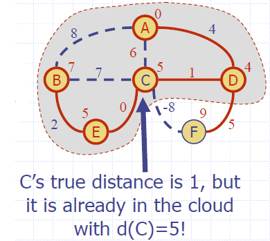
Why It Doesn’t Work for Negative-Weight Edges

Dijkstra’s algorithm is based on the greedy method. It adds vertices by increasing distance.
- If a node with a negative incident edge were to be added late to the cloud, it could mess up distances for vertices already in the cloud.

Shortest_Path_Dijkstra_Problem

Bellman-Ford Algorithm

Works even with negativeweight edges
Must assume directed edges (for otherwise we would have negativeweight cycles)
Iteration i finds all shortest paths that use i edges.
Running time: O(nm).
Can be extended to detect a negative-weight cycle if it exists
- How?

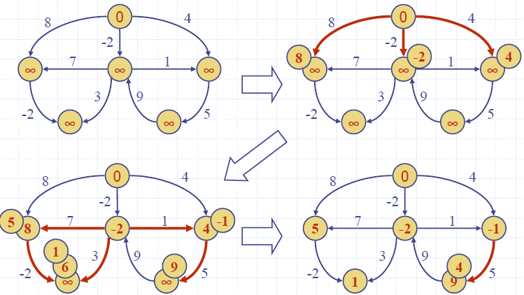
Algorithm BellmanFord(G, s)
for all v ∈ G.vertices()
  if v = s
    setDistance(v, 0)
  else
    setDistance(v, ∞)
  for i ← 1 to n-1 do
    for each e ∈ G.edges()
      { relax edge e }
      u ← G.origin(e)
      z ← G.opposite(u,e)
      r ← getDistance(u) + weight(e)
      if r < getDistance(z)
        setDistance(z,r)

Example

Bellmand Ford

DAG-based Algorithm

Works even with negative-weight edges
Uses topological order Doesn’t use any fancy data structures
Is much faster than Dijkstra’s algorithm
Running time: O(n+m).

Algorithm DagDistances(G, s)
  for all v ∈ G.vertices()
    if v = s
      setDistance(v, 0)
    else
      setDistance(v, ∞)
    Perform a topological sort of the vertices
    for u ← 1 to n do {in topological order}
      for each e ∈ G.outEdges(u)
        { relax edge e }
        z ← G.opposite(u,e)
        r ← getDistance(u) + weight(e)
        if r < getDistance(z)
          setDistance(z,r)

Example

Shortest_Path_DAG

All-Pairs Shortest Paths

Find the distance between every pair of vertices in a weighted directed graph G.
We can make n calls to Dijkstra’s algorithm (if no negative edges), which takes O(nmlog n) time.
Likewise, n calls to Bellman-Ford would take O(n²m) time.
We can achieve O(n³) time using dynamic programming (similar to the Floyd-Warshall algorithm).

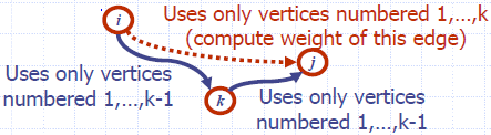
Algorithm AllPair(G) {assumes vertices 1,…,n}
  for all vertex pairs (i,j)
    if i = j
      D0[i,i] ← 0
    else if (i,j) is an edge in G
      D0[i,j] ← weight of edge (i,j)
    else
      D0[i,j] ← + ∞
  for k ← 1 to n do
    for i ← 1 to n do
      for j ← 1 to n do
      Dk[i,j] ← min{Dk-1[i,j], Dk-1[i,k]+Dk-1[k,j]}
  return Dn

Shortest_Path_All_Pairs_Shortest