Minimum Spanning Trees
Definition
- Spanning subgraph
- Subgraph of a graph G containing all the vertices of G
- Spanning tree
- Spanning subgraph that is itself a (free) tree
- Minimum spanning tree (MST)
- Spanning tree of a weighted graph with minimum total edge weight
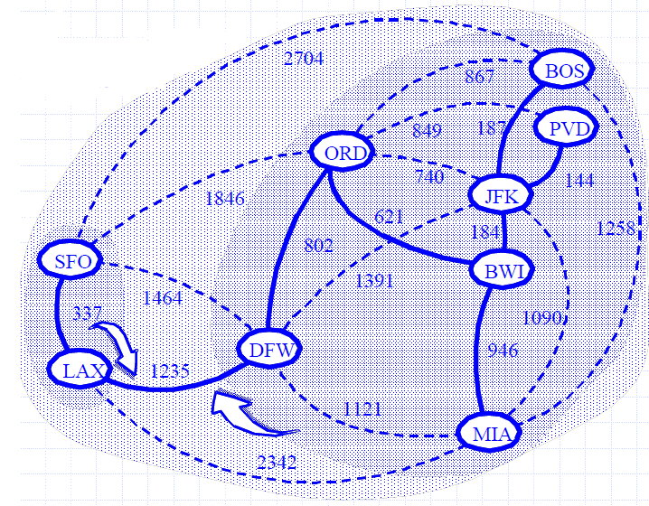
- Applications: Communications networks, Transportation networks
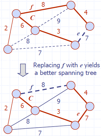
Cycle Property
- Let T be a minimum spanning tree of a weighted graph G
- Let e be an edge of G that is not in T and C let be the cycle formed by e with T
- For every edge f of C, weight(f) ≤ weight(e)
- Proof:
- By contradiction
- If weight(f) > weight(e) we can get a spanning tree of smaller weight by replacing e with f
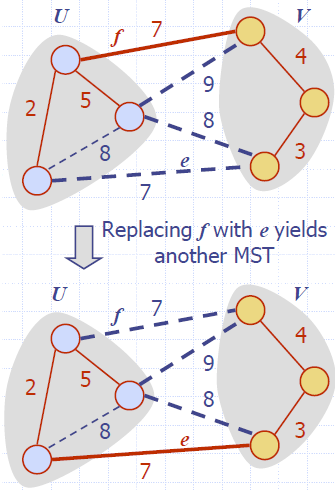
Partition Property
- Consider a partition of the vertices of G into subsets U and V
- Let e be an edge of minimum weight across the partition
- There is a minimum spanning tree of G containing edge e
- Proof:
- Let T be an MST of G
- If T does not contain e, consider the cycle C formed by e with T and let f be an edge of C across the partition
- By the cycle property, weight(f) ≤ weight(e)
- Thus, weight(f) = weight(e)
- We obtain another MST by replacing f with e
Prim-Jarnik’s Algorithm
- Similar to Dijkstra’s algorithm (for a connected graph)
- We pick an arbitrary vertex s and we grow the MST as a cloud of vertices, starting from s
- We store with each vertex v a label d(v) = the smallest weight of an edge connecting v to a vertex in the cloud
- At each step:
- We add to the cloud the vertex u outside the cloud with the smallest distance label
- We update the labels of the vertices adjacent to u
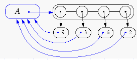
- A priority queue stores the vertices outside the cloud
- Key: distance
- Element: vertex
- Locator-based methods
- insert(k,e) returns a locator
- replaceKey(l,k) changes the key of an item
- We store three labels with each vertex:
- Distance
- Parent edge in MST
- Locator in priority queue
Algorithm PrimJarnikMST(G)
  Q ← new heap-based priority queue
  s ← a vertex of G
  for all v ∈ G.vertices()
    if v = s
      setDistance(v, 0)
    else
      setDistance(v, ∞)
    setParent(v, ∅)
    l ← Q.insert(getDistance(v), v)
    setLocator(v,l)
  while ¬Q.isEmpty()
    u ← Q.removeMin()
    for all e ∈ G.incidentEdges(u)
      z ← G.opposite(u,e)
      r ← weight(e)
      if r < getDistance(z)
        setDistance(z,r)
        setParent(z,e)
        Q.replaceKey(getLocator(z),r)
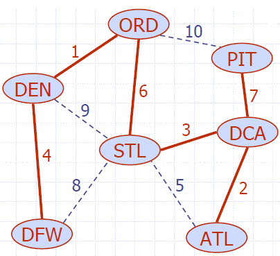
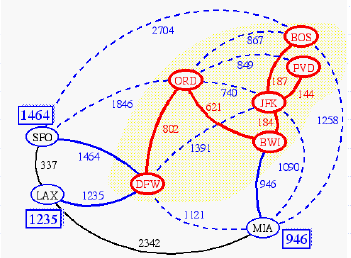
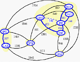
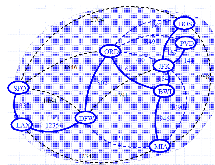
Example
Analysis
- Graph operations
- Method incidentEdges is called once for each vertex
- Label operations
- We set/get the distance, parent and locator labels of vertex z O(deg(z)) times
- Setting/getting a label takes O(1) time
- Priority queue operations
- Each vertex is inserted once into and removed once from the priority queue, where each insertion or removal takes O(log n) time
- The key of a vertex w in the priority queue is modified at most deg(w) times, where each key change takes O(log n) time
- Prim-Jarnik’s algorithm runs in O((n + m) log n) time provided the graph is represented by the adjacency list structure
- Recall that Σv deg(v) = 2m
- The running time is O(m log n) since the graph is connected
Kruskal’s Algorithm
- A priority queue stores the edges outside the cloud
- Key: weight
- Element: edge
- At the end of the algorithm
- We are left with one cloud that encompasses the MST
- A tree T which is our MST
Algorithm KruskalMST(G)
for each vertex V in G do
define a Cloud(v) of {v}
let Q be a priority queue.
Insert all edges into Q using their weights as the key
T ← ∅
while T has fewer than n-1 edges do
edge e = T.removeMin()
Let u, v be the endpoints of e
if Cloud(v) ≠ Cloud(u) then
Add edge e to T
Merge Cloud(v) and Cloud(u)
return T
Data Structure for Kruskal Algortihm
- The algorithm maintains a forest of trees
- An edge is accepted it if connects distinct trees
- We need a data structure that maintains a partition, i.e., a collection of disjoint sets, with the operations:
- find(u): return the set storing u
- union(u,v): replace the sets storing u and v with their union
Representation of a Partition
- Each set is stored in a sequence
- Each element has a reference back to the set
- operation find(u) takes O(1) time, and returns the set of which u is a member.
- in operation union(u,v), we move the elements of the smaller set to the sequence of the larger set and update their references
- the time for operation union(u,v) is min(nu,nv), where nu and nv are the sizes of the sets storing u and v
- Whenever an element is processed, it goes into a set of size at least double, hence each element is processed at most log n times
Partition-Based Implementation
- A partition-based version of Kruskal’s Algorithm performs cloud merges as unions and tests as finds.
- Running time: O((n+m)log n)
Algorithm Kruskal(G):
  Input: A weighted graph G.
  Output: An MST T for G.
  Let P be a partition of the vertices of G, where each vertex forms a separate set.
  Let Q be a priority queue storing the edges of G, sorted by their weights
  Let T be an initially-empty tree
  while Q is not empty do
    (u,v) ← Q.removeMinElement()
    if P.find(u) != P.find(v) then
      Add (u,v) to T
      P.union(u,v)
  return T
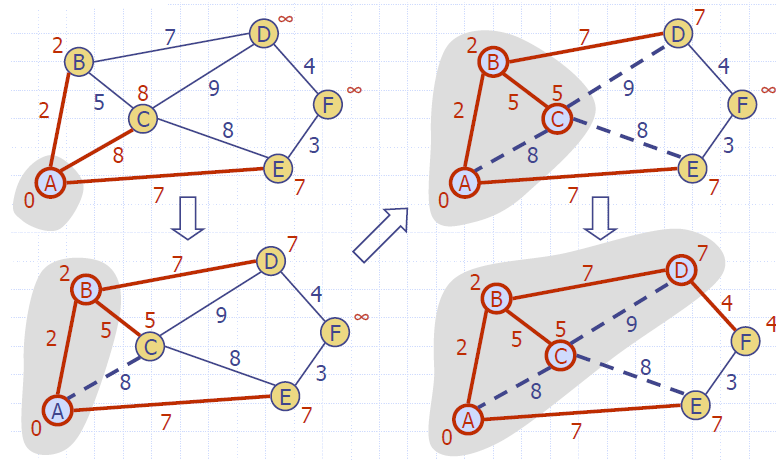
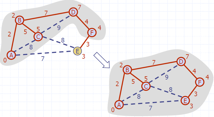
Example
Baruvka’s Algorithm
- Like Kruskal’s Algorithm, Baruvka’s algorithm grows many “clouds” at once.
- Each iteration of the while-loop halves the number of connected compontents in T.
- The running time is O(m log n).
Algorithm BaruvkaMST(G)
  T ← V {just the vertices of G}
  while T has fewer than n-1 edges do
    for each connected component C in T do
      Let edge e be the smallest-weight edge from C to another component in T.
      if e is not already in T then
        Add edge e to T
  return T
Example